Justice Inequality Simulator: Counterfactual Testing of a Court Outcome Model for Bias
1. Motivation
In May 2016, ProPublica published an investigation into COMPAS, a risk assessment tool used in the United States to predict whether a defendant will reoffend. Its main finding was that Black defendants who did not reoffend were classified as high risk at roughly twice the rate of white defendants who did not reoffend. Race was not an input of the tool. The bias came from the historical data the model learned from.
A year later, the Wisconsin Supreme Court ruled on this problem in State v. Loomis. Eric Loomis had been sentenced partly on the basis of a COMPAS score, and he could not see how the score was calculated because the method was a trade secret. The court allowed courts to keep using the tool, on condition that every report included a written warning about its limitations. The defendant still had no way to examine how his own score was produced.
Judicial risk prediction keeps running into the same issue. Historical sentencing data reflects the decisions of the judges, prosecutors and police who produced it. A model trained on that data reproduces those patterns in the form of a score, and a score is harder to contest than a person’s judgment because it looks objective. When the method is closed, the people affected by the score have very little to work with if they want to challenge it.
Most bias audits of these systems work at the group level: they compare error rates across race, gender or income and report the gap. This is useful, but it does not show which individual decisions depend on which words. I wanted to test something more direct: take one case, create a version where only one sensitive detail changes, and see whether the model’s prediction moves. If the predicted outcome changes only because a name or a pronoun changes, that is a concrete failure in a specific case.
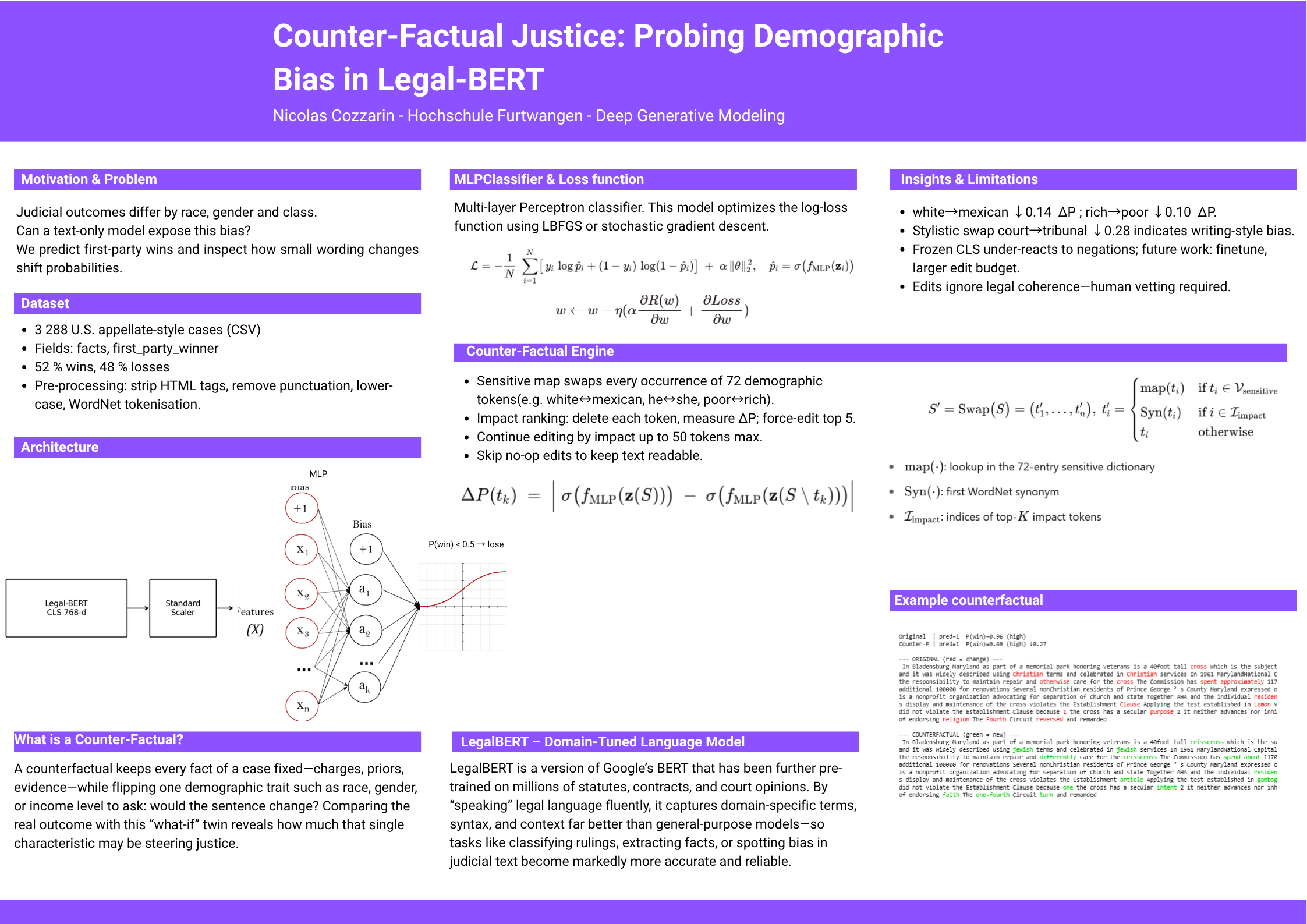
Goal: measure how sensitive a court-outcome prediction model is to sensitive attributes in the case text (gender, ethnicity and socioeconomic markers) by generating counterfactual versions of each case, and use that sensitivity as a case-level measure of bias in addition to group statistics.
2. Data
I considered three datasets:
| Source | Rows | Key features |
|---|---|---|
| COMPAS recidivism | ≈ 7,000 | age, priors, race, charge |
| U.S. Supreme Court Database (SCDB) | ≈ 28,000 | issue, petitioner, lower-court direction |
| justice.csv (U.S. Supreme Court cases, course data) | ≈ 5,000 | free-text facts, first_party_winner |
The method needs a text description of each case, so I used the third one, justice.csv. It contains U.S. Supreme Court cases with a short summary of the facts and a label saying whether the first party won. The other two datasets are mostly structured variables. The same method can be applied to any dataset that has a text description of the facts, with the preprocessing adapted to it.
Dataset and reference notebook: Supreme Court judgement prediction on Kaggle
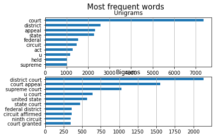
Figure 1: Most frequent words in the case descriptions
3. Preprocessing
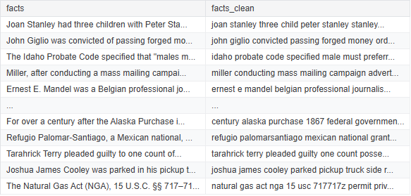
The case descriptions contain HTML tags, punctuation and extra whitespace. I remove them so that the model receives clean text, and I convert the outcome into a binary label.
import re
import pandas as pd

TAG_RE = re.compile(r"<[^>]+>")
PUNCT = str.maketrans("", "", r"""!"#$%&'()*+,-./:;<=>?@[]^_`{|}~""")

def clean(html: str) -> str:
    """Strip HTML and punctuation, and collapse whitespace."""
    text = TAG_RE.sub("", html or "").translate(PUNCT)
    return re.sub(r"\s+", " ", text).strip()

df = pd.read_csv("justice.csv").dropna(subset=["facts", "first_party_winner"])
df["text"] = df["facts"].map(clean)
df["label"] = (
    df["first_party_winner"]
    .astype(str).str.lower()
    .map({"true": 1, "false": 0, "1": 1, "0": 0})
)
Figure 2: Example of a cleaned record
4. Balancing the data
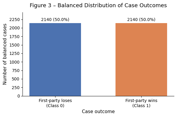
One outcome is more frequent than the other. Without a correction, a classifier can reach a good accuracy by predicting the majority outcome most of the time. I upsampled the minority class so that both outcomes have the same number of cases. Section 14 explains a problem with doing this before the train/test split.
from sklearn.utils import resample

pos = df[df.label == 1]
neg = df[df.label == 0]

minority = pos if len(pos) < len(neg) else neg
majority = neg if len(pos) < len(neg) else pos

minority_up = resample(
    minority,
    replace=True,
    n_samples=len(majority),
    random_state=42,
)

df_bal = pd.concat([majority, minority_up]).reset_index(drop=True)
Figure 3: Class distribution after balancing
5. Features with Legal-BERT
I convert each case description into a vector with Legal-BERT, a BERT model pre-trained on legal text. I use the hidden state of the [CLS] token as the representation of the whole text, which is the usual choice for classification. The embeddings are computed in batches, on GPU when available, and saved to disk so they do not have to be recomputed.
import numpy as np
import torch
from transformers import AutoTokenizer, AutoModel

DEVICE = "cuda" if torch.cuda.is_available() else "cpu"
MODEL_ID = "nlpaueb/legal-bert-base-uncased"

tok = AutoTokenizer.from_pretrained(MODEL_ID)
bert = AutoModel.from_pretrained(MODEL_ID).to(DEVICE).eval()

@torch.no_grad()
def embed(txts, batch=16, max_len=256):
    vecs = []
    for i in range(0, len(txts), batch):
        enc = tok(
            txts[i:i + batch],
            padding=True,
            truncation=True,
            max_length=max_len,
            return_tensors="pt",
        ).to(DEVICE)
        h = bert(**enc).last_hidden_state[:, 0]  # [CLS] token
        vecs.append(h.cpu())
    return torch.cat(vecs).numpy()

X = embed(df_bal.text.tolist())
np.save("legal_cls.npy", X)  # cache
Figure 4: t-SNE projection of the [CLS] embeddings, coloured by outcome
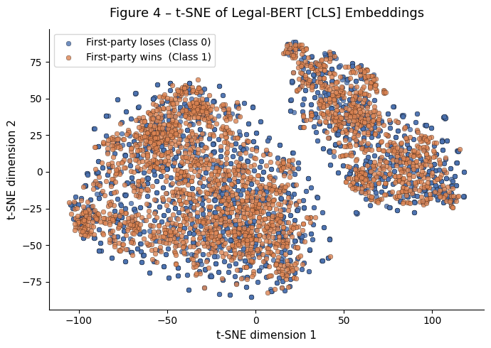
Figure 4 projects the 768-dimensional embeddings to two dimensions. Each dot is a case, and the colour shows whether the first party won or lost. The two outcomes are mixed together, and the two clusters that do appear are not related to the outcome. The pre-trained embeddings alone do not separate wins from losses, which makes the classifier’s job harder.
6. Scaling
I standardize the embeddings and multiply them by 5. The factor was meant to balance the text features against hand-crafted features in a later version; in this version there are no other features, so it only changes the scale of the input.
from sklearn.preprocessing import StandardScaler

scaler = StandardScaler().fit(X)
X_std = scaler.transform(X) * 5
7. Train, validation and test split
I split the data into 60 percent for training, 20 percent for validation and 20 percent for testing, keeping the same proportion of outcomes in each part.
from sklearn.model_selection import train_test_split

idx = np.arange(len(X_std))
train, tmp = train_test_split(
    idx, test_size=0.4, random_state=42, stratify=df_bal.label
)
val, test = train_test_split(
    tmp, test_size=0.5, random_state=42, stratify=df_bal.label.iloc[tmp]
)
8. Model
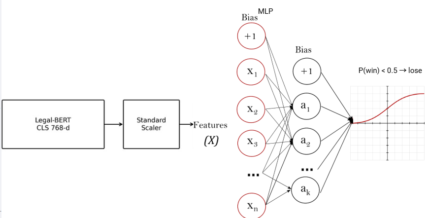
The classifier is a multi-layer perceptron with three hidden layers of 1024, 512 and 128 neurons on top of the 768-dimensional embeddings, with a sigmoid output for the binary outcome. Training stops early when the validation score stops improving.
from sklearn.neural_network import MLPClassifier

mlp = MLPClassifier(
    hidden_layer_sizes=(1024, 512, 128),
    activation="relu",
    alpha=1e-3,
    batch_size=128,
    max_iter=120,
    early_stopping=True,
    validation_fraction=0.20,
    n_iter_no_change=7,
    random_state=42,
)

mlp.fit(X_std[train], df_bal.label.iloc[train])
Figure 5: Model architecture
9. Training checks
I followed the training loss and compared the accuracy on the training, validation and test sets to check for overfitting.
import matplotlib.pyplot as plt
from sklearn.metrics import accuracy_score

plt.plot(mlp.loss_curve_)
plt.xlabel("Epoch")
plt.ylabel("Loss")
plt.title("MLP training loss")
plt.savefig("assets/2025-07-06-loss.png")

acc_train = accuracy_score(df_bal.label.iloc[train], mlp.predict(X_std[train]))
acc_val = accuracy_score(df_bal.label.iloc[val], mlp.predict(X_std[val]))
acc_test = accuracy_score(df_bal.label.iloc[test], mlp.predict(X_std[test]))
10. Counterfactual generator
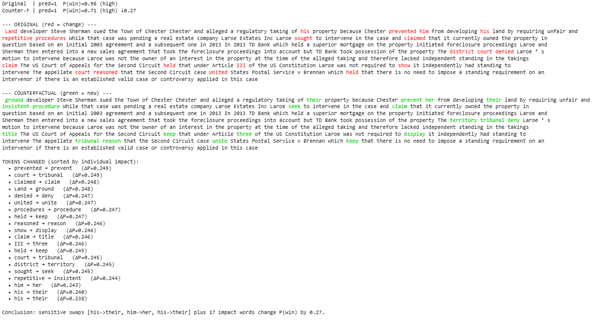
A counterfactual is a version of a case description with a few words changed and everything else kept the same. Comparing the model’s prediction on the original and on the counterfactual shows which words the prediction depends on. The generator works in three steps:
- Swap every sensitive word that has a pair in the mapping (for example “he” and “she”).
- Swap a fixed number of the words with the highest influence on the prediction (TOP_FORCE).
- Keep swapping influential words until a maximum number of edits is reached (TOP_K).
def build_cf(i):
    w = toks(texts[i])
    changed, sens = set(), []
    impacts = impact_map(i)

    # 1) swap sensitive tokens (skip no-ops)
    for p, t in enumerate(w):
        if t.lower() in SENSITIVE_MAP:
            new = subst(t)
            if new != t:
                w[p] = new
                changed.add(p)
                sens.append((t, new))

    # 2) force TOP_FORCE swaps among the most influential tokens
    imp_sorted = sorted(impacts.items(), key=lambda x: x[1], reverse=True)
    forced = 0
    for p, _ in imp_sorted:
        if forced >= TOP_FORCE:
            break
        if p not in changed:
            new = subst(w[p])
            if new != w[p]:
                w[p] = new
                changed.add(p)
                forced += 1

    # 3) continue until TOP_K edits
    for p, _ in imp_sorted:
        if len(changed) >= min(TOP_K, len(w)):
            break
        if p not in changed:
            new = subst(w[p])
            if new != w[p]:
                w[p] = new
                changed.add(p)

    return " ".join(w), changed, sens, impacts
Figure 6: Example of a counterfactual
The full code is in the Colab notebook linked at the end of this article.
11. Measuring sensitivity
The idea behind the test is simple: if a model is fair with respect to an attribute, its prediction should not change when only that attribute changes in the text.
For each case, I compute the predicted probability that the first party wins, build the counterfactual with build_cf, and compute the probability again. The difference between the two is the model’s sensitivity for that case. Because the generator also records which tokens were swapped and how much each one influenced the prediction, the test also shows which words drove the change.
This measure is local: it describes the behaviour of the model on one case. Group metrics describe averages over many cases. The two answer different questions, and an audit needs both.
12. Results
| Metric | Value |
|---|---|
| Accuracy (test) | 0.78 |
| ROC-AUC (test) | 0.84 |
I examined the counterfactuals case by case with an interactive loop:
- Swaps of gendered words moved the predicted probability by more than 0.05.
- Substitutions of sensitive words often moved it by 0.10 to 0.25.
- The shifts were larger when words related to the sensitive term were also changed.
- Some cases did not change at all.
This suggests that in some cases the prediction depends on wording linked to gender, ethnicity or socioeconomic status, even though none of these attributes is an input of the model. Section 14 explains why these numbers are indicative rather than final.
13. Discussion
The training loss levels off and the validation and test accuracies are similar, so the model does not show strong overfitting. Accuracy, however, says nothing about whether the prediction depends on sensitive wording, which is what the counterfactual test is for.
Two improvements would make the predictions more reliable for an audit. Cases whose embedding is more than three standard deviations from the training mean could be flagged as uncertain, so the model reports low confidence instead of a precise-looking number. Temperature scaling would make the predicted probabilities better calibrated, which matters when the measure of bias is a change in probability.
Future work could replace the MLP with a generative model such as a conditional VAE or a cGAN, which could generate counterfactuals that read more naturally than word swaps, and expose the system through a REST API.
14. Limits of this evaluation
Reviewing the project later, I found three issues that a reader should keep in mind.
Upsampling before the split. I upsampled the minority class (section 4) before splitting the data (section 7). Upsampling copies cases, so the same case can appear in both the training set and the test set. The model has then already seen part of the test data, and the accuracy of 0.78 and the ROC-AUC of 0.84 are probably optimistic. The correct order is to split first and balance only the training set, or to use class weights instead of copies.
Edits that are not sensitive. Steps 2 and 3 of the generator also change the most influential words, even when they are not sensitive. In those counterfactuals, part of the shift comes from these extra edits. To attribute a change to gender or ethnicity, the measurement should use counterfactuals with only the sensitive swaps.
Case-by-case inspection. The shifts in section 12 come from inspecting examples, not from a run over the whole test set. A stronger result would report the average and the distribution of the shift over all test cases, separately for each type of swap. Simple word swaps can also change the meaning of a sentence (for example “white” in “white car”), so the swap list needs to be checked in context.
These issues concern how the method was evaluated in this project, not the idea of counterfactual testing itself.
15. Policy and governance relevance
This project is a small academic version of a question that courts and governments are already facing: what happens when part of a judicial decision depends on a model trained on a history that is not neutral.
The COMPAS investigation and State v. Loomis show two sides of the problem. ProPublica’s finding came from comparing error rates between groups, which a single accuracy score would not have shown. A counterfactual test looks for the same kind of problem in individual cases. Loomis shows that even when a court has doubts about a tool, it may have no way to examine a specific decision because the method is proprietary. A counterfactual test does not need access to the model’s internals: it only needs the ability to change an input and observe the output. A court, a regulator or a journalist can run it on a system they do not control.
Two European texts point in the same direction. Article 22 of the GDPR gives individuals the right not to be subject to a decision based solely on automated processing that has legal effects on them, without safeguards. The EU AI Act classifies AI systems that assist judicial authorities in researching and interpreting facts and law as high risk (Recital 61 and Annex III), because of “the risks of potential biases, errors and opacity.” Both texts require systems whose decisions can be examined and contested. The counterfactual method is one practical way to examine them.
A class project does not settle these questions. Building a small audit tool did help me understand what these legal requirements ask engineers to do in practice.
16. References
- COMPAS dataset (ProPublica)
- Supreme Court Database (Washington University, Olin School of Law)
- Angwin, J., Larson, J., Mattu, S., Kirchner, L., “Machine Bias,” ProPublica, 2016
- State v. Loomis, 881 N.W.2d 749, 2016 WI 68 (Wis. 2016)
- European Union, General Data Protection Regulation, Article 22
- European Union, Artificial Intelligence Act, Recital 61 and Annex III, point 8, on high-risk classification for AI assisting judicial authorities
- Devlin et al., “BERT: Pre-training of Deep Bidirectional Transformers,” 2018
- CEUR-WS Vol-3841, Paper 5: Counterfactual Explanations in Legal NLP
- HFU Deep Generative Models lecture notes
This project started as a project proposal for Ruxandra Lasowski’s Deep Generative Models class in the HFU Master’s programme.
Source code: Google Colab notebook